An Introduction to Climate Technology and Geoengineering

What would it actually take to stop the Earth from warming? And, beyond that, could we remove enough carbon from the atmosphere to undo some of the warming we have already caused?

What interests me about these questions is that they connect a planetary problem to a set of physical processes we can begin to understand. Sunlight arrives, heat escapes, carbon moves between reservoirs. Human activity has altered these processes, but understanding the changes gives us a way to examine what might be done about them.

This essay begins with a simple model of the Earth’s energy balance, then follows carbon through the atmosphere, land and ocean. From there, I want to look at the technologies available to reduce emissions, remove carbon dioxide and change how much sunlight the Earth absorbs. These interventions act on different parts of the system. Understanding those differences is essential to judging what each could achieve.

My focus is primarily technical, rather than a survey of climate policy. But a technology’s energy requirements, environmental effects and need for long-term management are part of its feasibility, not details we can leave until after the engineering is finished. I am optimistic about the possibilities here; I also think the most useful optimism begins with being clear about what a calculation does—and does not—tell us.

Originally published in June 2020. Historical scenarios and dated assessments are identified below.

Basic radiative equilibrium

The simplest place to begin is with an energy budget. For the Earth’s climate to remain broadly stable over time, the rate at which the planet absorbs energy must match the rate at which it loses energy to space. If more arrives than leaves, energy accumulates in the system, much of it in the ocean.

This is a balance of energy, not temperature. A watt is a joule of energy per second; a flux measured in watts per square metre tells us how quickly energy crosses a given area. Temperature is one consequence of how that energy is stored and distributed.

We can construct a useful first approximation from just a few quantities. NASA’s explanation of the Earth’s energy budget provides a more detailed account of the processes behind it.

Incoming sunlight

At the Earth’s distance from the Sun, a surface facing the Sun directly receives roughly 1,360 watts per square metre at the top of the atmosphere. Call this solar irradiance $S_0$.

The Earth intercepts sunlight over a circular area, but that energy is distributed over a sphere with four times the area. Averaging across the whole planet therefore gives us $S_0/4$.

Not all of that sunlight is absorbed. Clouds, atmospheric particles, ice and other surfaces reflect some of it back to space. The fraction reflected is the Earth’s albedo, represented by $\alpha$, with an approximate planetary average of 0.30.

Bringing these together, the globally averaged absorbed solar flux is:

The rounded inputs give 238 watts per square metre; 240 is a useful approximation. This is the energy absorbed by the Earth system as a whole, not just by its surface.

Outgoing heat and the greenhouse effect

The Earth also emits energy as thermal infrared radiation. We can define an effective emission temperature, $T_{\mathrm{em}}$, using the Stefan–Boltzmann relationship:

Here, $\sigma$ is the Stefan–Boltzmann constant, approximately $5.67 \times 10^{-8}\,\mathrm{W\,m^{-2}\,K^{-4}}$. At equilibrium, incoming and outgoing fluxes are equal, so:

That is about −18°C. Yet a familiar rounded reference for the Earth’s average surface temperature is around 288 K, or 15°C. Why the difference?

The calculation gives us the temperature associated with radiation escaping to space, not the temperature of the ground or ocean beneath the atmosphere. Greenhouse gases—including water vapour, carbon dioxide and methane—absorb infrared radiation and emit it in all directions. Some returns towards the surface; some travels upwards, where it may be absorbed and emitted again.

The atmosphere is not equally transparent at every wavelength, so energy escapes from different heights, including directly from the surface in some parts of the spectrum. Much of it leaves from atmospheric layers colder than the surface. The surface can therefore be warmer than the effective emission temperature while the planet still loses the required amount of energy to space.

Convection and evaporation help connect these layers. Warm air rises; evaporating water carries energy away from the surface; condensation releases that energy into the atmosphere. Radiation and convection together shape the temperature profile of the lower atmosphere, or troposphere. This is the basis of radiative-convective equilibrium. Convection moves energy within the system; radiation is still how the planet ultimately loses energy to space.

A useful way to picture the relationship is:

Here, $T_s$ is surface temperature, $\Gamma$ is an approximate rate of temperature decline with height, and $z_{\mathrm{em}}$ is an illustrative effective emission height. A decline of 6.5 K per kilometre over 5 kilometres gives a surface roughly 33 K warmer than the emitting level.

This helps explain the gap between 255 K and 288 K. It is not an independent prediction of the surface temperature: the lapse rate and emission height are assumptions, and neither is a single fixed value for the real atmosphere.

What additional greenhouse gases change

Adding CO₂ makes the atmosphere more opaque to infrared radiation in the wavelengths it absorbs. Initially, with temperatures otherwise unchanged, less energy escapes to space. The Earth gains energy until warming increases outgoing radiation enough to restore balance, with feedbacks affecting the size of the adjustment.

Water vapour is an important part of this response. A warmer atmosphere can contain more water vapour, which strengthens the greenhouse effect and amplifies the initial warming. Melting snow and ice can also expose darker surfaces, increasing absorbed sunlight. These are positive feedbacks: they reinforce an initial change. The terms positive and negative describe the direction of a feedback, not whether it is desirable.

The basic mechanism is worth keeping in mind. Fossil fuels do not warm the planet chiefly because burning them releases heat. They add greenhouse gases that change how efficiently the Earth can lose energy it receives from the Sun.

The carbon cycle

We have described a flow of energy. Carbon follows a different budget: it moves between the atmosphere, living organisms, soils, oceans and rocks. The two budgets are connected because the amount of atmospheric CO₂ affects the Earth’s energy balance, but they are not interchangeable.

A stock is the amount of carbon in a reservoir; a flow is the amount transferred over a period of time. A forest can take up a large amount of carbon through photosynthesis while returning almost as much through respiration and decomposition. The difference between those flows determines whether its carbon stock is growing.

Units matter here. A gigatonne, or Gt, is a billion metric tonnes. GtC measures the mass of carbon alone; GtCO₂ includes the oxygen in carbon dioxide. One tonne of carbon corresponds to approximately 3.67 tonnes of CO₂. Atmospheric concentration, usually expressed in parts per million or ppm, is another quantity again: the proportion of air molecules that are CO₂.

NASA’s account of the carbon cycle is a useful guide to these reservoirs and their different timescales. Its historical statistics should be read in the context of its 2011 publication.

Land: growth, respiration and storage

Plants use sunlight to turn CO₂ and water into organic matter through photosynthesis. Some of this carbon becomes leaves, wood and roots; some passes into soils, animals and microorganisms.

Carbon also returns to the atmosphere. Plants respire, microorganisms decompose organic matter, and fires release stored carbon. Decomposition occurs in both oxygen-rich and oxygen-poor conditions; the latter can also produce methane. Most dead plant material returns to the active cycle rather than becoming fossil fuel.

The important quantity is therefore not simply how much carbon plants absorb, but how much remains stored after these losses. Forests matter, but so do soils, peatlands and the conditions that allow their carbon stocks to persist.

Higher CO₂ concentrations can stimulate plant growth and increase carbon storage. Where that slows the rise of atmospheric CO₂, it is a negative feedback on the original increase. It is not unlimited: nutrients, water, temperature and available land constrain growth, while drought, fire and mortality can return carbon to the atmosphere. The IPCC’s assessment of carbon-cycle feedbacks examines these competing effects.

Oceans: chemistry, circulation and life

CO₂ dissolves into surface seawater and participates in a set of chemical reactions. Much of the ocean’s dissolved inorganic carbon exists as bicarbonate, alongside carbonate ions and dissolved CO₂. Circulation carries carbon-rich water into the ocean interior, where its return to contact with the atmosphere can take centuries or longer.

Biology adds another route. Phytoplankton use dissolved inorganic carbon to grow. Some organic material sinks after organisms die or are eaten, carrying carbon into deeper water. Much is broken down and recycled; only a fraction reaches long-lived sediment storage. This is the biological pump, distinct from the physical and chemical processes that also drive ocean uptake.

By absorbing some of our emissions, the ocean limits the rise in atmospheric CO₂. But the chemistry has consequences. Adding CO₂ increases hydrogen-ion concentrations and lowers pH, while reducing the availability of carbonate ions used by many shell-building organisms. The ocean remains alkaline overall, but becomes more acidic. NOAA’s explanation of ocean acidification sets out this distinction.

The ocean is not an unlimited sink. Its uptake depends on temperature, circulation and chemical buffering, among other factors. Warming generally reduces CO₂ solubility, and biological responses complicate the picture further. It would be a mistake to treat natural absorption as a fixed disposal service that will expand to match whatever we emit.

Rocks, fossil fuels and the geological cycle

Over much longer timescales, weathering, sediment burial, plate tectonics and volcanic activity move carbon between the surface and the Earth’s crust and interior. Some silicate-weathering reactions consume CO₂; carbon can eventually enter sediments and rocks. Subduction carries carbon-bearing material downwards, while geological processes also return CO₂ to the atmosphere.

Fossil fuels form where a small fraction of organic matter is preserved, buried and transformed over geological time. Burning coal, oil and natural gas transfers that ancient carbon back into the active cycle very quickly. Changes in land use add further emissions by reducing or disturbing existing carbon stores.

This difference in timescales is central to the problem. We are releasing carbon accumulated over millions of years much faster than geological processes can take it back.

The animation below, by Robert Rohde, shows how human activity perturbs the carbon cycle. It is a historical visualisation, not a live carbon budget. Its stocks are measured in GtC and its annual flows in GtC per year.

Source: Robert Rohde, via Berkeley Earth: The Earth’s Carbon Cycle.

Why the accumulation matters

Large natural flows do not make human emissions unimportant. What matters is their net effect. Land and ocean absorb some of the additional carbon, but not enough to prevent atmospheric CO₂ from rising.

CO₂ also has no single useful atmospheric expiry date. Some of an emission is taken up relatively quickly; other parts of its perturbation persist for centuries to many thousands of years as carbon moves through the system. It is not a pollutant that simply washes out shortly after we turn off the source.

A bathtub is a useful, if incomplete, analogy. Reducing the flow from the tap can slow the rise in water level without making the level fall. Similarly, reducing annual CO₂ emissions is not the same as removing the carbon already accumulated. The complication is that the Earth’s ‘drain’ is not fixed: land and ocean uptake changes as concentrations and climate change.

There is a close relationship between cumulative human CO₂ emissions and the warming they cause. This is why climate discussions focus on a carbon budget—the total additional emissions compatible with a specified warming limit and probability—rather than only on the emissions of a particular year.

Addressing the issue

The physical problem now has a clearer shape. We need to limit further accumulation, reduce the effects of other greenhouse gases and, if we want to bring CO₂-driven warming down again, achieve sustained net removal.

That does not mean every response serves the same purpose. Reducing emissions prevents an addition to the problem. Carbon dioxide removal takes carbon out of the atmosphere and stores it. Solar radiation modification attempts to reduce warming by changing the incoming-energy side of the budget, without removing the CO₂. Adaptation—such as preparing cities for heat or improving flood protection—reduces harm, but does not itself resolve the planetary energy imbalance.

Temperature goals are about reducing risk

The Paris Agreement, adopted in 2015, aims to hold warming well below 2°C above pre-industrial levels while pursuing efforts to limit it to 1.5°C. These are not boundaries separating a harmless climate from a uniformly disastrous one. Risks generally increase with each additional increment of warming, and particular ecosystems or physical systems have their own thresholds and vulnerabilities.

As a dated point of reference, the World Meteorological Organization’s assessment of 2025 put that year’s global mean temperature at about 1.43°C above the 1850–1900 average. Its assessment of 2024 put the previous year at about 1.55°C. An individual year above 1.5°C is not the same as reaching that level of sustained warming, which is assessed over longer periods. Year-to-year variability sits on top of the long-term trend.

A global average also conceals substantial regional differences. Land generally warms more than ocean, and the Arctic warms faster than the global average. The consequences depend on where people live, the systems they rely on and their capacity to respond—not just on the global number.

What net zero means

Net-zero CO₂ means balancing remaining human-caused CO₂ emissions with human-caused removals over a specified period. It approximately stops further CO₂-driven global warming. This is not the same as immediately returning temperatures to their pre-industrial level, and it does not settle the effects of methane, nitrous oxide or other climate drivers. Net-zero CO₂ and net-zero greenhouse gases are different accounting goals.

The existing natural land and ocean sinks cannot simply be counted again as an additional offset: their uptake is already part of the system’s response to our emissions. Nor does net zero mean maintaining present emissions and building a removal industry of equal size. The IPCC’s Sixth Assessment synthesis emphasises deep reductions in gross emissions, with removals counterbalancing the residual emissions that remain difficult to eliminate.

The timing matters because cumulative emissions matter. Two pathways can reach net zero in the same year while producing very different amounts of warming if one emits much more on the way there. A distant endpoint is not a substitute for reducing the flow now.

Pathways and the problem of overshoot

The 2018 IPCC special report was the basis of the original version of this essay. Its four illustrative pathways remain useful for understanding the choices within a model, provided we do not mistake them for forecasts of what will happen.

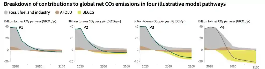
P1 explored a world with lower energy demand, rapid emissions reductions and no reliance on bioenergy with carbon capture and storage, or BECCS. P2 combined sustainable consumption, low-carbon innovation and land management with more limited BECCS. P3 followed a more conventional development trajectory and relied more heavily on removals. P4 assumed resource- and energy-intensive development, with a large temperature overshoot and extensive later use of BECCS.

The useful lesson is not that one diagram tells us how much of a particular machine to build. It is that assumptions about demand, land use and the speed of emissions reductions strongly affect how much later removal a pathway requires.

The assessments also need to be kept separate. The 2018 report described 1.5°C pathways with no or limited overshoot as reducing net CO₂ emissions by about 45% from 2010 levels by 2030. In the 2023 synthesis, assessed pathways limiting warming to 1.5°C with more than 50% likelihood and no or limited overshoot had median 2030 reductions of 48% for CO₂ and 43% for all greenhouse gases, relative to 2019, with global net-zero CO₂ in the early 2050s. These are characteristics of dated modelled pathways, not a timetable that restarts whenever the report is read.

An overshoot pathway exceeds a temperature level before returning below it, generally through sustained net-negative CO₂ emissions. But bringing the global average temperature back down would not automatically restore a lost ecosystem, reverse every change in an ice sheet or undo the sea-level rise experienced in the meantime. The size and duration of overshoot matter, and relying on more future removal adds its own feasibility and sustainability risks.

That is the context in which I think the technologies should be examined: what can they do, what would delivering that result require, and how much are we assuming about their future availability?

Climate technology starts with emissions reduction

Before looking at ways to remove carbon, it is worth considering the work we can avoid creating. Keeping a tonne of fossil CO₂ out of the atmosphere avoids the need to separate that same carbon from dilute air later, transport it and find somewhere to store it.

For many activities, the approach is to use less energy for the same service, electrify the process where practical and supply that electricity from low-carbon sources. Insulation reduces the heating a building needs. Heat pumps move heat rather than producing it directly from fuel. Electric motors can replace combustion engines. Renewable generation and other low-carbon electricity sources reduce the emissions associated with powering these systems.

These are interconnected changes. An electric vehicle’s benefit depends in part on the electricity used to charge it and the emissions involved in making it. A power system with substantial wind and solar needs ways to match supply and demand, including transmission, storage, flexible demand and dependable generation. Comparing a single device without the system around it can give a misleading picture.

Other activities are harder to change. Cement production releases CO₂ through chemical reactions as well as energy use. Aviation, shipping and some industrial processes face constraints that differ from those of a household appliance. Low-carbon fuels, changes in materials and processes, and carbon capture may each have a role, with different costs and limits. The IPCC’s mitigation assessment considers this wider set of options.

It is important to distinguish carbon capture at a fossil or industrial source from carbon removal. Capturing fossil CO₂ before it is released primarily avoids an emission; it does not remove the accumulated CO₂ already in the air. Capturing atmospheric carbon and storing it durably is a different service. Both can be useful, but they should not be credited as the same intervention.

I do not see the less novel technologies as a preliminary step to the interesting ones. Every reduction in emissions changes the scale of the removal problem we would otherwise have to solve.

Carbon dioxide removal

Carbon dioxide removal, or CDR, deliberately takes CO₂ from the atmosphere and stores it in vegetation, soils, geological formations, minerals or other reservoirs. It can counterbalance residual emissions; if total removals exceed remaining emissions, it can also contribute to gradually reducing CO₂-driven warming.

The phrase covers very different processes. A tonne stored in a growing forest does not have the same reversal risk as a tonne mineralised or injected into a well-selected geological formation. Nor is a tonne captured necessarily a tonne removed once energy use, materials, transport and subsequent releases are included.

The National Academies’ assessment of negative emissions provides a useful framework for these differences. For any proposal, I would want to ask:

• Additionality: how much extra removal happens because of the intervention, compared with what would have happened without it?
• Net benefit: what emissions are created across the project’s full life cycle?
• Storage: where does the carbon go, how long is it expected to remain there, and what could release it?
• Verification: what is measured, what is modelled, and how much uncertainty remains?
• Scale: what land, energy, materials, infrastructure and continuing management would be required?

These questions give us a way to compare technologies without assuming that all claimed tonnes are equivalent.

Forests, soils and the limits of biological storage

Restoring forests can increase carbon held in vegetation and soils while providing benefits for habitats, water and local communities. Protecting an existing forest can prevent emissions from its destruction. Those are both valuable, but preventing a loss and creating an additional sink are different outcomes.

Biological storage is also vulnerable to reversal. Fire, drought, disease, clearing or a change in management can return carbon to the atmosphere. Growth eventually slows, and land is needed for food, settlements and ecosystems as well as carbon storage. Planting trees everywhere is not a general solution: the effects depend on the location, the previous ecosystem and changes in reflectivity and water exchange, as well as carbon uptake.

I think these approaches are important precisely because they work with living systems we depend on for more than carbon. That is also why it would be a mistake to judge them only by a short-term tonnes-per-hectare target, or to treat their storage as interchangeable with permanent disposal of fossil carbon.

Protecting frozen carbon: Pleistocene Park

A related, but different, objective is to prevent carbon already stored in the ground from being released. Pleistocene Park, in north-eastern Siberia, explores whether restoring populations of large grazing animals can help protect permafrost.

The mechanism is more specific than simply replacing dark forest with bright grassland. Snow insulates the ground during winter. Animals disturb and compact it, potentially allowing more heat to escape from the soil into the cold air. Grazing also changes vegetation, which affects reflectivity, summer insulation and the carbon balance.

A 2020 study combining field observations with modelling found evidence for the snow-compaction mechanism and explored its potential across the Arctic. Its large-scale results depended on assumptions about widespread changes in snow conditions associated with high animal densities. They were not a demonstration that those conditions could be achieved sustainably across the region.

I find this an interesting example of how an apparently indirect intervention—changing the animals in a landscape—could affect a physical process beneath it. But the climate case depends on the full ecological and seasonal balance, not on the novelty of the idea. It is experimental ecosystem management aimed at avoiding future permafrost emissions, not demonstrated atmospheric carbon removal or a reason to clear Arctic forests.

Bioenergy with carbon capture and storage

BECCS combines two processes. Plants take up atmospheric CO₂ as they grow; biomass is then used to produce energy, and some of the resulting CO₂ is captured and stored rather than released.

In principle, this transfers carbon from the atmosphere into geological storage while supplying useful energy. In practice, whether the result is net-negative depends on where the biomass comes from, what would otherwise have happened to the land and material, the emissions from growing and transporting it, the capture rate and the storage system.

Using a waste stream is not the same proposition as establishing a large energy-crop plantation. Large-scale demand for biomass can compete with food production, water and biodiversity, or cause land-use changes that undermine the intended benefit. This is why the substantial BECCS quantities in some model pathways need scrutiny: a model’s use of a technology is not evidence that its assumed scale will be environmentally or socially achievable.

Direct air capture

Direct air capture, or DAC, separates CO₂ from ambient air. In common approaches, air contacts a chemical solvent or solid sorbent that binds CO₂. The material is then regenerated, using heat, pressure changes or a combination of inputs, to release a concentrated CO₂ stream for reuse or storage.

For durable removal, capture is only the beginning. The CO₂ must be stored in a way that keeps it out of the atmosphere. Turning it into a fuel that is soon burned may recycle carbon, but does not provide the same durable removal service as geological storage or mineralisation.

The attraction of DAC is that it does not depend on a nearby concentrated emissions source. A plant can, within practical limits, be located around suitable energy and storage resources. The difficulty is that CO₂ is dilute in air: a great deal of material has to be contacted to collect a relatively small amount of it.

How much work must separation require? For an idealised gas mixture, the reversible minimum work per mole for extracting a very small fraction of the available CO₂ into a pure stream at the same temperature and pressure is approximately:

Here, $R$ is the molar gas constant, $T$ is absolute temperature and $x_{\mathrm{CO_2}}$ is the CO₂ mole fraction. Using 298 K and a rounded 400 ppm for illustration gives about 19–20 kilojoules per mole, or roughly 120 kilowatt-hours per tonne of CO₂. Extracting a larger fraction from each air stream raises the minimum. House and colleagues’ thermodynamic analysis explains the fuller separation calculation and its limitations.

If that work could be supplied as electricity at an assumed US$0.05 per kilowatt-hour, the idealised separation energy bill would be about US$6 per tonne. That is not the cost of delivering a tonne of carbon removal.

The distinction is substantial. Real equipment needs finite flow rates and driving forces. Fans overcome pressure losses; capture materials must be regenerated and replaced; concentrated CO₂ may need further compression, transport and injection. Equipment, finance, maintenance and storage monitoring also cost money. Approaching reversible operation can require larger equipment, so lower energy use does not necessarily mean lower total cost. The minimum is a measure of work, not an interchangeable allowance of electricity and low-temperature heat.

For comparison, a 2018 process study by Keith and colleagues estimated US$94–232 per tonne captured for a particular proposed plant, depending on its assumptions. That was a process-design estimate, not an observed price for verified net removal. Neither it nor the idealised US$6 energy bill should be treated as a current market quotation.

We can still use arithmetic to make the scale concrete. A programme delivering one gigatonne of net removal per year at an assumed US$200 per tonne would cost US$200 billion annually. Both the removal rate and unit cost are assumptions, not a forecast. The programme would also need to build and operate the capture, energy, transport and storage infrastructure required for a billion tonnes every year.

The source of that energy matters. A project’s own emissions reduce its net benefit, and clean energy used for capture has alternative uses, including displacing fossil generation. Likewise, removing a given mass of CO₂ does not produce a fixed, one-for-one decline in atmospheric concentration: land and ocean exchanges respond to the change.

I see a serious reason to develop DAC, particularly for residual emissions and eventual net-negative emissions. But the thermodynamic calculation establishes a physical lower bound. It does not establish that large-scale cleanup will be cheap or quick.

Enhanced weathering

Another approach begins with the geological processes discussed earlier. Some silicate minerals react in ways that consume CO₂. Enhanced weathering aims to accelerate these processes by increasing the surface area of reactive rock and placing it in conditions where weathering can occur more quickly.

The original example that interested me was Project Vesta’s proposal to use crushed olivine in coastal environments. As the mineral dissolves, it can add alkalinity to seawater, changing the carbonate chemistry so the water can subsequently take up additional atmospheric CO₂. The durable carbon storage is largely in dissolved forms, rather than simply in a newly formed pile of solid carbonate.

There are two separate steps here: dissolving the mineral and drawing additional CO₂ across the air–sea boundary. We cannot assume that applying a tonne of rock immediately completes both. Mineral composition, grain size, temperature, water movement, secondary reactions and gas exchange affect the amount and timing of removal. A 2025 review of coastal olivine weathering examines these mechanisms and the difficulty of verifying the result.

On land, crushed basalt can be spread on agricultural soils, with weathering products potentially carried through groundwater and rivers towards longer-lived storage. This is related chemistry, but a different setting; evidence for one approach does not automatically establish the performance of the other.

There is encouraging field research. A four-year Illinois trial published in 2024 applied basalt at 50 tonnes per hectare annually and reported cumulative CO₂ removal potential of 10.5 ± 3.8 tonnes per hectare, inferred from the release of calcium and magnesium from the rock. The researchers explicitly distinguished that estimate from directly measuring all subsequent transport and storage effects. It is evidence of weathering under field conditions, not proof that every inferred tonne had already reached permanent storage—or validation of coastal olivine economics.

The practical questions are substantial. Finer grinding can speed reactions but uses energy. Mining, transport and spreading create costs and emissions. Some minerals contain metals such as nickel that require environmental assessment. In an open coastal system, distinguishing additional atmospheric uptake from what the ocean would have absorbed anyway requires observations and modelling, not just a record of how much rock was delivered.

This is why I would not treat a low mining cost, or a theoretical quantity of CO₂ consumed per tonne of pure mineral, as the price of verified removal. The chemistry gives us a reason to investigate. Delivering an additional, durable and environmentally acceptable result is the engineering and measurement problem that follows.

Solar radiation modification

Carbon removal acts on the atmospheric carbon stock. Solar radiation modification, or SRM, acts on a different part of the system: how much incoming sunlight is absorbed. The term geoengineering has been used to cover both, but grouping them together can obscure how differently they work.

Recall the energy-balance calculation. If the Earth’s albedo increases, absorbed sunlight decreases. Holding everything else fixed, a change in albedo produces:

An illustrative increase in planetary albedo from 0.30 to 0.31 would therefore reduce absorbed sunlight by about 3.4 watts per square metre. This is a calculation of flux, not a prediction of a particular temperature reduction. The response would depend on feedbacks, timescales and where and how the intervention occurred.

Stratospheric aerosols

One widely studied proposal is to introduce particles, or gases that form particles, into the stratosphere so they scatter some incoming sunlight back to space. Other proposals include changing the reflectivity of certain marine clouds; they have different mechanisms and uncertainties.

The natural example most often used to explain stratospheric aerosols is the 1991 eruption of Mount Pinatubo in the Philippines. Sulfur dioxide injected high into the atmosphere formed sulfate aerosols. The resulting reduction in solar heating contributed to temporary global cooling of roughly half a degree over the following few years, as described by the US Geological Survey.

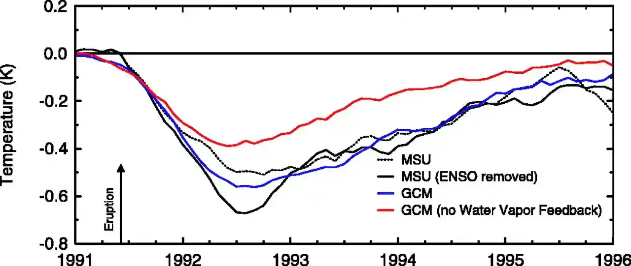
Source: Soden and colleagues, Global Cooling After the Eruption of Mount Pinatubo.

The eruption demonstrates that stratospheric aerosols can cool the climate. It does not demonstrate that maintaining an artificial aerosol layer would safely reproduce an earlier climate. Cooling by reducing sunlight does not reverse all the effects of warming caused by greenhouse gases, especially across different regions and seasons.

What cooling would leave unresolved

SRM does not remove CO₂. It therefore does not directly solve CO₂-driven ocean acidification, and matching a global average temperature would not necessarily restore previous rainfall patterns or other regional conditions. Aerosols can also affect stratospheric chemistry and ozone.

Their short atmospheric lifetime creates a further obligation. If an intervention supplied substantial cooling while greenhouse gas concentrations remained high, suddenly stopping it could expose the world to rapid warming as the aerosols disappeared. The IPCC’s assessment of solar radiation modification identifies this termination risk. A material that disappears relatively quickly is not the same as an intervention whose consequences can be safely switched off.

Who would decide the amount of cooling? How would competing regional interests be represented? Who would monitor the effects, manage interruption risks and remain responsible across political changes? These are not incidental objections to an otherwise complete technical design. They are requirements of operating a planetary intervention.

I think there is a serious case for research into the physical effects, risks and governance of SRM. The National Academies’ Reflecting Sunlight report makes an important distinction between studying the subject and endorsing deployment. Understanding an option—including discovering that particular approaches are unacceptable—is valuable. Assuming that it will be available to compensate for delayed emissions reductions is a very different proposition.

Conclusion

I began with two questions: how could we stop further warming, and could we eventually undo some of it? Working through the system makes the answers more specific.

Deep emissions reductions and net-zero CO₂ address the continuing accumulation of carbon, alongside reductions in other greenhouse gases. Durable carbon removal could counterbalance residual emissions and, if sustained beyond them, gradually reduce CO₂-driven warming. Solar radiation modification could alter the energy balance more quickly, but would leave important causes and consequences of the problem unresolved and introduce continuing management risks. None of these gives us a general way to restore everything already lost.

Personally, I remain optimistic about the role of technological innovation. There is room to improve materials, processes, energy systems and the ways we measure and verify results. There is also value in investigating unconventional ideas, provided we can distinguish an interesting mechanism from evidence that it works at the scale proposed.

Cost reductions will matter, but so will the incentives to pay for an outcome whose benefits are widely shared. A technology can be physically effective without having a viable route to deployment; a commercially successful product can also deliver less climate benefit than its headline numbers suggest. The technical, economic and institutional questions have to meet somewhere, even when an essay begins with the physics.

What I find most encouraging is that the problem becomes more concrete as we understand it. We can ask which flow an intervention changes, where the carbon goes, what resources are required and what evidence would establish success. The more clearly we can answer those questions, the better placed we are to turn an interesting idea into a useful climate technology.

Thank you for reading.

Any views expressed here are mine only and do not reflect any current or former employer.

References

Climate physics and the carbon cycle

• NASA Earth Observatory (2009), Climate and Earth’s Energy Budget. The energy-budget explanation; detailed estimates reflect its publication context.
• NASA Earth Observatory (2011), The Carbon Cycle. Fast and slow carbon-cycle mechanisms; not a source of current concentration or emissions figures.
• NOAA, Ocean acidification. Carbonate chemistry and consequences for marine organisms.
• IPCC (2021), AR6 Working Group I, Chapter 5: Global Carbon and Other Biogeochemical Cycles and Feedbacks. Carbon sinks, persistence and feedbacks.
• Rohde, R., The Earth’s Carbon Cycle, Berkeley Earth. Source and attribution for the historical animation.

Temperature goals and mitigation pathways

• UNFCCC, The Paris Agreement. Official description of the agreement and its temperature goals.
• WMO (2025; 2026), State of the Global Climate 2024 and State of the Global Climate 2025. Annual observations and their distinction from long-term warming.
• IPCC (2018), Global Warming of 1.5°C, Summary for Policymakers, especially C.1–C.3 and Figure SPM.3b. Historical pathways and their assumptions.
• IPCC (2023), AR6 Synthesis Report, Summary for Policymakers, especially B.5–B.7 and Table SPM.1. Carbon budgets, net zero, mitigation pathways and overshoot.
• IPCC (2022), AR6 Working Group III, Summary for Policymakers, especially C.3–C.5 and C.11. Emissions reductions, CDR, storage and sustainability constraints.

Carbon removal and ecosystem interventions

• National Academies of Sciences, Engineering, and Medicine (2019), Negative Emissions Technologies and Reliable Sequestration: Summary. Removal mechanisms, land constraints, permanence and verification.
• Beer, C. and colleagues (2020), Protection of Permafrost Soils from Thawing by Increasing Herbivore Density, Scientific Reports. Field observations and a model experiment, not demonstrated Arctic-scale deployment.
• House, K. Z. and colleagues (2011), Economic and energetic analysis of capturing CO₂ from ambient air, PNAS. Separation thermodynamics and the distinction between minimum work and actual system requirements; its historical price projections are not used as current prices here.
• Keith, D. W. and colleagues (2018), A Process for Capturing CO₂ from the Atmosphere, Joule. A specific process-design and cost estimate, not a verified net-removal market price.
• Beerling, D. J. and colleagues (2024), Enhanced weathering in the US Corn Belt delivers carbon removal with agronomic benefits, PNAS. Basalt field-trial results and the limits of the reported removal-potential accounting.
• Geerts, L. J. J., Hylén, A. and Meysman, F. J. R. (2025), Review and syntheses: Ocean alkalinity enhancement and carbon dioxide removal through marine enhanced rock weathering using olivine, Biogeosciences. Coastal weathering mechanisms, dissolution and verification challenges.

Solar radiation modification

• US Geological Survey (1997), The Cataclysmic 1991 Eruption of Mount Pinatubo, Philippines. Sulfur emissions, aerosols and temporary cooling.
• Soden, B. J. and colleagues (2002), Global Cooling After the Eruption of Mount Pinatubo: A Test of Climate Feedback by Water Vapor, Science. Source of the lower-tropospheric temperature figure.
• IPCC (2021), AR6 Working Group I, Chapter 4: Future Global Climate, especially §4.6.3.3. Solar radiation modification and termination risks.
• National Academies of Sciences, Engineering, and Medicine (2021), Reflecting Sunlight: Summary. Research, uncertainty and governance; not an endorsement of deployment.