Radioactivity and Neutron Interactions

Navigation #

1. Introduction
2. Radioactive decay rates
     2.1 Unit of measurement for radioactivity
     2.2 Variation of radioactivity over time
3. Radioactive half-life
4. Plotting radioactive decay
     4.1 Multiple radioactive nuclides
5. Radioactive equilibrium
6. Transient radioactive equilibrium
7. Neutron scattering
      7.1 Elastic
      7.2 Inelastic
8. Fission
9. References

Introduction

In the previous post, we learned that atoms that do not have stable nuclei work towards a stable configuration. In order to do so, they undergo a variety of transformational processes classified as radioactive decay. Though the decay of radioactive nuclides occurs in a random manner, studies have revealed that we can assign a certain probability that a certain fraction of the nuclei within any given nuclide will decay. The final section of this post will focus on the concept of ‘neutron interactions’ which will lead into the concept of fission, a process integral to nuclear physics and the operation of nuclear reactors.

Radioactive decay rates

The probability introduced above is known as the radioactive decay constant, $\lambda$. This constant is given as a probability per unit time i.e. 1/second, 1/minute or 1/year. This constant is used to calculate what is known as the activity $(A)$ of a sample—the number of disintegrations per second. Equation 1 below outlines how this number is calculated:

$$A=\lambda N$$

Equation 1

Where:
$A$ = Activity of the nuclide (disintegrations/second)
$\lambda$ = Decay constant of the nuclide (second^-1)
$N$ = Number of atoms of the nuclide in the sample

Unit of measurement for radioactivity

Two common units used to measure the activity of a substance are the Curie $(C_i)$ and becquerel $(B_q)$. A becquerel is equal to 1 disintegration per second and is used in the metric system, while a curie is used in the United States and is approximately $3.7\times {10}^{10}$ becquerels.

Variation of radioactivity over time

From equation 1 above, it is possible to derive an expression (outside of the scope of this essay) to calculate how the number of atoms present will change over time:

$$N=N_o{e}^{-\lambda t}$$

Equation 2

Where:
$N$ = Number of atoms present at time t
$N_o$ = Number of atoms initially present
$\lambda$ = Decay constant (time^-1)
$t$ = Time

Since activity and number of atoms are always proportional, The following can be used to describe the activity at a given time:

$$A=A_o{e}^{-\lambda t}$$

Equation 3

Where:
$A$ = Activity present at time t
$A_o$ = Activity initially present
$\lambda$ = Decay constant (time^-1)
$t$ = Time

Radioactive half-life

A concept that defines the amount of time required for the radioactive activity to decrease to one-half of its original value is known as the radioactive half-life. This is a highly useful number which is calculated by solving calculation 3 for the time, t, when the current activity, A, equals one-half the initial activity A_o:

$$t_{1/2}=\frac{ln2}{\lambda }=\frac{0.693}{\lambda }$$

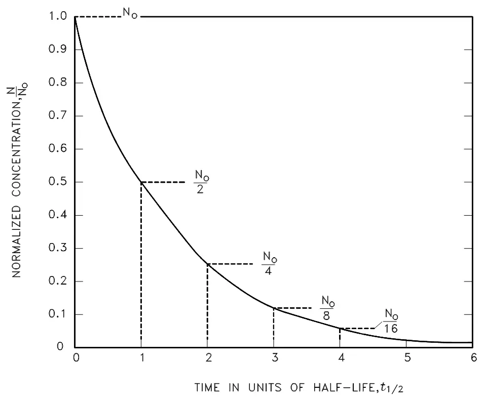
Figure 1. Radioactive decay as a function of time in units of half-life.

Plotting radioactive decay

As we see in figure 1, it can be useful to plot the activity of a nuclide as it changes over time. We can show similar decay curves, on both linear or logarithmic scales, against time in seconds as opposed to in half-life units. For example, we may be given the following problem and data:

• Plot the radioactive decay curve for Nitrogen-16 over a period of 100 seconds:
  • Initial activity is 142 curies;
  • The half-life of Nitrogen-16 is 7.13 seconds.

First, solve for the decay constant, given the half-life:

$$\begin{array}{rl}{t}_{1/2}& =\frac{0.693}{\lambda }\\ \lambda & =\frac{0.693}{t_{1/2}}\\ \lambda & =\frac{0.693}{7.13seconds}\\ \lambda & =0.0972secon{d}^{-1}\end{array}$$

$$t_{1/2}=\frac{0.693}{\lambda }$$
$$\lambda =\frac{0.693}{t_{1/2}}$$
$$\lambda =\frac{0.693}{7.13seconds}$$
$$\lambda =0.0972secon{d}^{-1}$$

Now use the decay constant above to calculate the activity at various times, using equation 3:

$$A=A_o{e}^{-\lambda t}$$

Table 1. Data points for Nitrogen-16 decay.

Plotting the data points in the table above yields the following plots:

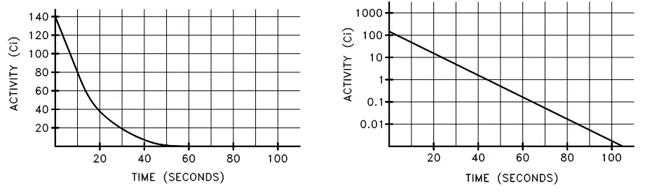
Figure 2. Linear and semi-log plots of Nitrogen-16 decay.

Multiple radioactive nuclides

What if a substance has multiple radioactive nuclides? In that case, the total activity is the sum of the individual activities of each nuclide. Consider the following sample:

• $1\times {10}^6$ atoms of iron-25 with a half-life of 44.51 days $(\lambda =1.80\times {10}^{7}se{c}^{-1})$
• $1\times {10}^6$ atoms of manganese-54 with a half-life of 312.2 days $(\lambda =2.57\times {10}^{-8}se{c}^{-1})$
• $1\times {10}^6$ atoms of cobalt-60 with a half-life of 1925 days $(\lambda =4.17\times {10}^{-9}se{c}^{-1})$

The intial activity of each of the nuclides would be the product of the number of atoms and the decay constant:

$$\begin{array}{rl}{A}_{Fe-50}& =N_{Fe-59}{\lambda }_{Fe-59}\\ & =(1\times {10}^{6}atoms)(1.80\times {10}^{-7}se{c}^{-1})\\ & =0.180Ci\end{array}$$

$$\begin{array}{rl}{A}_{Mn-54}& =N_{Mn-54}{\lambda }_{Mn-54}\\ & =(1\times {10}^{6}atoms)(2.57\times {10}^{-8}se{c}^{-1})\\ & =0.0257Ci\end{array}$$

$$\begin{array}{rl}{A}_{Fe-50}& =N_{Fe-59}{\lambda }_{Fe-59}\\ & =(1\times {10}^{6}atoms)(4.17\times {10}^{-9}se{c}^{-1})\\ & =0.00417Ci\end{array}$$

When we plot the decay of these three nuclides, initially we see that the activity of the shortest-lived nuclide (Iron-59) dominates the total activity, then Manganese-54 dominates. After almost all of the iron and manganese have decayed away, the only contributor to activity will be the Cobalt-60 as seen in figure 3 below:

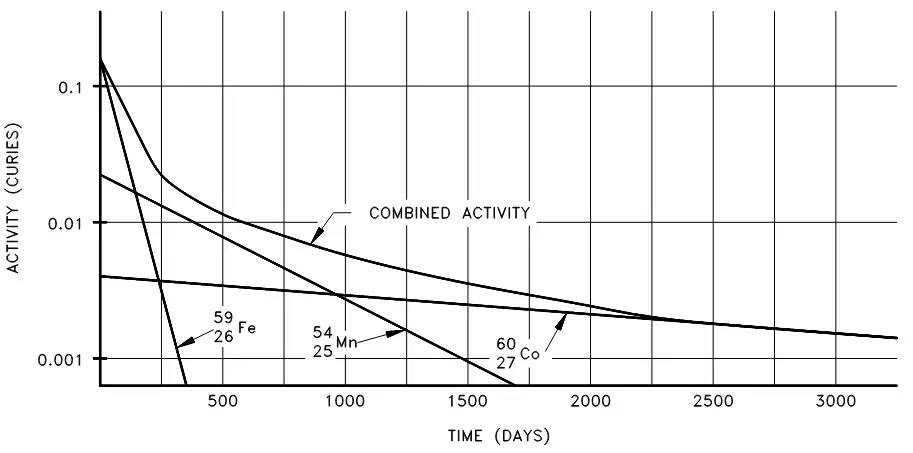
Figure 3. Combined decay of Iron-56, Manganese-54 and Cobalt-60.

Radioactive equilibrium

Radioactive equilibrium exists when a radioactive nuclide is decaying at the same rate at which it is being produced. From what we have learned so far, we know that as the amount of a given radioactive substance increases, the rate of decay will increase proportionally (given the decay constant). Imagine, then, production of an unstable isotope of sodium-24, which decays at a half-life of 14.96 hours and is initially produced at $1\times {10}^6$ atoms per second:

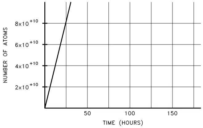
Figure 4. Cumulative production of sodium-24 over time.

Initially, the sodium-24 increases rapidly, then will increase at a continually diminishing rate until the rate of decay is equal to the rate of production. We can use the equation below to set the production rate (R) to be equal to the decay rate $(\lambda N)$:

$$R=\lambda N\therefore N=\frac{R}{\lambda }$$

Equation 4

Where:
$R$ = Production rate (atoms/second)
$\lambda$ = Decay constant (second^-1)
$N$ = Number of atoms

If we wanted to calculate the equilibrium value for sodium-24 being produced at the rate of $1\times {10}^6$ atoms per second we could do the following:

$$\begin{array}{rl}\lambda & =\frac{0.693}{t_{1/2}}\\ & =\frac{0.693}{14.96hours}(\frac{1hour}{3600seconds})\\ & =1.287\times {10}^{-5}secon{d}^{-1}\end{array}$$

And:

$$\begin{array}{rl}N& =\frac{R}{\lambda }\\ & =\frac{1\times {10}^6:\frac{atoms}{second}}{1.287\times {10}^{-5}secon{d}^{-1}}\\ & =7.77\times {10}^{10}atoms\end{array}$$

Equation 5 below can be used to calculate the values of the amount of sodium-24 present at different times, though the development of the equation is again outside the scope of this series:

$$N=\frac{R}{\lambda }(1-e^{-\lambda t})$$

Equation 5

A plot of the approach of sodium-24 to equilibrium is shown in figure 5 below:

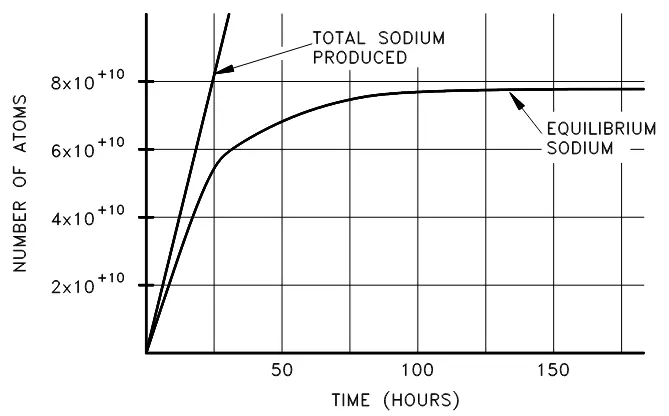
Figure 5. Approach of sodium-24 to equilibrium.

Transient radioactive equilibrium

Transient radioactive equilibrium occurs when the parent and daughter nuclide decay at essentially the same rate. For such an equilibrium to occur, the parent must have a long half-life when compared to the daughter. An example is barium-140, which decays by beta emission to lanthanum-140, which decays by beta emission to stable cerium-140 as seen in the decay chain below:

Although the decay constant for barium-140 is smaller, the actual rate of decay $(\lambda N)$ is initially larger than that of lanthanum-140 because of the great difference in their initial concentrations. As the concentration of the daughter increases, the rate of decay of the daughter will approach and eventually match the decay rate of the parent. When this occurs, they are said to be in transient equilibrium. A plot of the barium-lanthanum-cerium decay chain reaching transient equilibrium is shown in Figure 6:

Figure 6. Transient equilibrium in the decay of barium-140.

Secular equilibrium occurs when the parent has an extremely long half-life. Where all of the elements in a long decay chain are in secular equilibrium, each of the descendants has built up to an equilibrium amount and all decay at the rate set by the original parent; the only exception being the final stable element on the end of the chain, which has a constantly increasing number of atoms.

Neutron scattering

Of special interest to nuclear engineers are nuclear reactions caused by incident neutrons or reactions that produce neutrons. One such reaction is that of neutron scattering:

When two nuclei interact and produce one or more products, while conserving a number of quantities (examined in the previous post), this is known as a binary reaction. Scattering is one type of these binary reactions, occurring when the projectile and target product are the same. Neutron scattering occurs when a nucleus, after having been struck by a neutron, emits a single neutron. The net result of such an interaction is as if the projectile neutron had merely ‘bounced off’, or scattered from, the nucleus. These can either be:

Elastic

No energy is transferred into nuclear excitation and the target nucleus is left in the ground state.

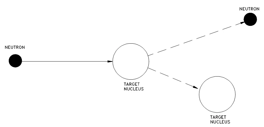
Figure 7. Elastic scattering.

Such elastic scattering can occur in two ways. Typically it will be through potential elastic scattering, essentially billiard balls with impenetrable surfaces. Here, the neutron does not touch the nucleus, the neutron is acted on and scattered by the short-range nuclear forces as it approaches the nucleus. The more unusual case is that of resonance elastic scattering whereby the neutron is actually absorbed, a compound nucleus forms, and a neutron is re-emitted such that the total kinetic energy is conserved and the nucleus returns to the ground state.

Inelastic

In this case, the incident neutron is absorbed by the target nucleus, forming a compound nucleus that will use some of the incident kinetic energy to emit a neutron of lower kinetic energy, leaving the original nucleus in an excited state. This nucleus will usually decay rapidly through the emission of a gamma photon, once or a number of times until it reaches the ground state.

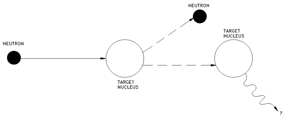
Figure 8. Inelastic scattering.

Here, the initial kinetic energy of the projectile neutron is equal to the sum of the kinetic energy of the exit neutron, the target nucleus, and the total gamma energy.

Fission

Scattering is one possible type of interaction a neutron can cause. Another is absorption, whereby the neutron is absorbed into the nucleus, resulting in the loss of a neutron coupled with the production of a gamma-ray, a subatomic particle or it may cause the nucleus to fission.

In an earlier post discussing binding energy, we saw that nuclear energy can be obtained by splitting a nucleus (preferably a heavy one) into two lighter nuclei. This is a fission reaction and is an important and practical source of energy, which will be discussed in more detail in the next post.

References

• Department of Energy. (2015). DOE Fundamentals Handbook, Nuclear Physics and Reactor Theory, Volume 1 of 2 [Ebook]. Retrieved 28 December 2020, from https://www.standards.doe.gov/standards-documents/1000/1019-bhdbk-1993-v1.
• Shultis, J., & Faw, R. (2005). Fundamentals of nuclear science and engineering. CRC Press.